Artificial Intelligence Nanodegree
Convolutional Neural Networks
Project: Write an Algorithm for a Dog Identification App
Why We're Here
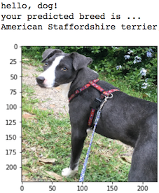
In this notebook, you will make the first steps towards developing an algorithm that could be used as part of a mobile or web app. At the end of this project, your code will accept any user-supplied image as input. If a dog is detected in the image, it will provide an estimate of the dog's breed. If a human is detected, it will provide an estimate of the dog breed that is most resembling. The image below displays potential sample output of your finished project (... but we expect that each student's algorithm will behave differently!).
In this real-world setting, you will need to piece together a series of models to perform different tasks; for instance, the algorithm that detects humans in an image will be different from the CNN that infers dog breed. There are many points of possible failure, and no perfect algorithm exists. Your imperfect solution will nonetheless create a fun user experience!
The Road Ahead
We break the notebook into separate steps. Feel free to use the links below to navigate the notebook.
- Step 0: Import Datasets
- Step 1: Detect Humans
- Step 2: Detect Dogs
- Step 3: Create a CNN to Classify Dog Breeds (from Scratch)
- Step 4: Use a CNN to Classify Dog Breeds (using Transfer Learning)
- Step 5: Create a CNN to Classify Dog Breeds (using Transfer Learning)
- Step 6: Write your Algorithm
- Step 7: Test Your Algorithm
Step 0: Import Datasets
Import Dog Dataset
In the code cell below, we import a dataset of dog images. We populate a few variables through the use of the load_files function from the scikit-learn library:
train_files,valid_files,test_files- numpy arrays containing file paths to imagestrain_targets,valid_targets,test_targets- numpy arrays containing onehot-encoded classification labelsdog_names- list of string-valued dog breed names for translating labels
from sklearn.datasets import load_files
from keras.utils import np_utils
import numpy as np
from glob import glob

# define function to load train, test, and validation datasets
def load_dataset(path):
    data = load_files(path)
    dog_files = np.array(data['filenames'])
    dog_targets = np_utils.to_categorical(np.array(data['target']), 133)
    return dog_files, dog_targets

# load train, test, and validation datasets
train_files, train_targets = load_dataset('dogImages/train')
valid_files, valid_targets = load_dataset('dogImages/valid')
test_files, test_targets = load_dataset('dogImages/test')

# load list of dog names
dog_names = [item[20:-1] for item in sorted(glob("dogImages/train/*/"))]

# print statistics about the dataset
print('There are %d total dog categories.' % len(dog_names))
print('There are %s total dog images.\n' % len(np.hstack([train_files, valid_files, test_files])))
print('There are %d training dog images.' % len(train_files))
print('There are %d validation dog images.' % len(valid_files))
print('There are %d test dog images.'% len(test_files))
Import Human Dataset
In the code cell below, we import a dataset of human images, where the file paths are stored in the numpy array human_files.
import random
random.seed(8675309)

# load filenames in shuffled human dataset
human_files = np.array(glob("lfw/*/*"))
random.shuffle(human_files)

# print statistics about the dataset
print('There are %d total human images.' % len(human_files))
Step 1: Detect Humans
We use OpenCV's implementation of Haar feature-based cascade classifiers to detect human faces in images. OpenCV provides many pre-trained face detectors, stored as XML files on github. We have downloaded one of these detectors and stored it in the haarcascades directory.
In the next code cell, we demonstrate how to use this detector to find human faces in a sample image.
import cv2
import matplotlib.pyplot as plt
%matplotlib inline

# extract pre-trained face detector
face_cascade = cv2.CascadeClassifier('haarcascades/haarcascade_frontalface_alt.xml')

# load color (BGR) image
img = cv2.imread(human_files[3])
# convert BGR image to grayscale
gray = cv2.cvtColor(img, cv2.COLOR_BGR2GRAY)

# find faces in image
faces = face_cascade.detectMultiScale(gray)

# print number of faces detected in the image
print('Number of faces detected:', len(faces))

# get bounding box for each detected face
for (x,y,w,h) in faces:
    # add bounding box to color image
    cv2.rectangle(img,(x,y),(x+w,y+h),(255,0,0),2)

# convert BGR image to RGB for plotting
cv_rgb = cv2.cvtColor(img, cv2.COLOR_BGR2RGB)

# display the image, along with bounding box
plt.imshow(cv_rgb)
plt.show()

Before using any of the face detectors, it is standard procedure to convert the images to grayscale. The detectMultiScale function executes the classifier stored in face_cascade and takes the grayscale image as a parameter.
In the above code, faces is a numpy array of detected faces, where each row corresponds to a detected face. Each detected face is a 1D array with four entries that specifies the bounding box of the detected face. The first two entries in the array (extracted in the above code as x and y) specify the horizontal and vertical positions of the top left corner of the bounding box. The last two entries in the array (extracted here as w and h) specify the width and height of the box.
Write a Human Face Detector
We can use this procedure to write a function that returns True if a human face is detected in an image and False otherwise. This function, aptly named face_detector, takes a string-valued file path to an image as input and appears in the code block below.
# returns "True" if face is detected in image stored at img_path
def face_detector(img_path):
    img = cv2.imread(img_path)
    gray = cv2.cvtColor(img, cv2.COLOR_BGR2GRAY)
    faces = face_cascade.detectMultiScale(gray)
    return len(faces) > 0
(IMPLEMENTATION) Assess the Human Face Detector
Question 1: Use the code cell below to test the performance of the face_detector function.
- What percentage of the first 100 images in
human_fileshave a detected human face? - What percentage of the first 100 images in
dog_fileshave a detected human face?
Ideally, we would like 100% of human images with a detected face and 0% of dog images with a detected face. You will see that our algorithm falls short of this goal, but still gives acceptable performance. We extract the file paths for the first 100 images from each of the datasets and store them in the numpy arrays human_files_short and dog_files_short.
Answer:
human_files_short = human_files[:100]
dog_files_short = train_files[:100]
# Do NOT modify the code above this line.

## TODO: Test the performance of the face_detector algorithm
## on the images in human_files_short and dog_files_short.
true_positives = sum([1 for x in human_files_short if face_detector(x)])
false_positives = sum([1 for x in dog_files_short if face_detector(x)])

print "Human Detected in human_files: {:.1f}%\nHuman Detected in dog_files: {:.1f}%".format((float(true_positives)/len(human_files_short))*100, (float(false_positives)/len(dog_files_short))*100)
Question 2: This algorithmic choice necessitates that we communicate to the user that we accept human images only when they provide a clear view of a face (otherwise, we risk having unneccessarily frustrated users!). In your opinion, is this a reasonable expectation to pose on the user? If not, can you think of a way to detect humans in images that does not necessitate an image with a clearly presented face?
Answer:
This is a clear and reasonable requirement for the end user to submit pictures with a clear view of the subject. If there is not a clear view of the face, it can be vague for both humans and machines attempting to classify the subject. It's important to set expectations for machine vision applications because of the compute, gpu, and memory constraints associated with building the software.
We suggest the face detector from OpenCV as a potential way to detect human images in your algorithm, but you are free to explore other approaches, especially approaches that make use of deep learning :). Please use the code cell below to design and test your own face detection algorithm. If you decide to pursue this optional task, report performance on each of the datasets.
## (Optional) TODO: Report the performance of another
## face detection algorithm on the LFW dataset
### Feel free to use as many code cells as needed.
Step 2: Detect Dogs
In this section, we use a pre-trained ResNet-50 model to detect dogs in images. Our first line of code downloads the ResNet-50 model, along with weights that have been trained on ImageNet, a very large, very popular dataset used for image classification and other vision tasks. ImageNet contains over 10 million URLs, each linking to an image containing an object from one of 1000 categories. Given an image, this pre-trained ResNet-50 model returns a prediction (derived from the available categories in ImageNet) for the object that is contained in the image.
from keras.applications.resnet50 import ResNet50

# define ResNet50 model
ResNet50_model = ResNet50(weights='imagenet')
Pre-process the Data
When using TensorFlow as backend, Keras CNNs require a 4D array (which we'll also refer to as a 4D tensor) as input, with shape
$$ (\text{nb_samples}, \text{rows}, \text{columns}, \text{channels}), $$
where nb_samples corresponds to the total number of images (or samples), and rows, columns, and channels correspond to the number of rows, columns, and channels for each image, respectively.
The path_to_tensor function below takes a string-valued file path to a color image as input and returns a 4D tensor suitable for supplying to a Keras CNN. The function first loads the image and resizes it to a square image that is $224 \times 224$ pixels. Next, the image is converted to an array, which is then resized to a 4D tensor. In this case, since we are working with color images, each image has three channels. Likewise, since we are processing a single image (or sample), the returned tensor will always have shape
$$ (1, 224, 224, 3). $$
The paths_to_tensor function takes a numpy array of string-valued image paths as input and returns a 4D tensor with shape
$$ (\text{nb_samples}, 224, 224, 3). $$
Here, nb_samples is the number of samples, or number of images, in the supplied array of image paths. It is best to think of nb_samples as the number of 3D tensors (where each 3D tensor corresponds to a different image) in your dataset!
from keras.preprocessing import image
from tqdm import tqdm

def path_to_tensor(img_path):
    # loads RGB image as PIL.Image.Image type
    img = image.load_img(img_path, target_size=(224, 224))
    # convert PIL.Image.Image type to 3D tensor with shape (224, 224, 3)
    x = image.img_to_array(img)
    # convert 3D tensor to 4D tensor with shape (1, 224, 224, 3) and return 4D tensor
    return np.expand_dims(x, axis=0)

def paths_to_tensor(img_paths):
    list_of_tensors = [path_to_tensor(img_path) for img_path in tqdm(img_paths)]
    return np.vstack(list_of_tensors)
Making Predictions with ResNet-50
Getting the 4D tensor ready for ResNet-50, and for any other pre-trained model in Keras, requires some additional processing. First, the RGB image is converted to BGR by reordering the channels. All pre-trained models have the additional normalization step that the mean pixel (expressed in RGB as $[103.939, 116.779, 123.68]$ and calculated from all pixels in all images in ImageNet) must be subtracted from every pixel in each image. This is implemented in the imported function preprocess_input. If you're curious, you can check the code for preprocess_input here.
Now that we have a way to format our image for supplying to ResNet-50, we are now ready to use the model to extract the predictions. This is accomplished with the predict method, which returns an array whose $i$-th entry is the model's predicted probability that the image belongs to the $i$-th ImageNet category. This is implemented in the ResNet50_predict_labels function below.
By taking the argmax of the predicted probability vector, we obtain an integer corresponding to the model's predicted object class, which we can identify with an object category through the use of this dictionary.
from keras.applications.resnet50 import preprocess_input, decode_predictions

def ResNet50_predict_labels(img_path):
    # returns prediction vector for image located at img_path
    img = preprocess_input(path_to_tensor(img_path))
    return np.argmax(ResNet50_model.predict(img))
Write a Dog Detector
While looking at the dictionary, you will notice that the categories corresponding to dogs appear in an uninterrupted sequence and correspond to dictionary keys 151-268, inclusive, to include all categories from 'Chihuahua' to 'Mexican hairless'. Thus, in order to check to see if an image is predicted to contain a dog by the pre-trained ResNet-50 model, we need only check if the ResNet50_predict_labels function above returns a value between 151 and 268 (inclusive).
We use these ideas to complete the dog_detector function below, which returns True if a dog is detected in an image (and False if not).
### returns "True" if a dog is detected in the image stored at img_path
def dog_detector(img_path):
    prediction = ResNet50_predict_labels(img_path)
    return ((prediction <= 268) & (prediction >= 151))
(IMPLEMENTATION) Assess the Dog Detector
Question 3: Use the code cell below to test the performance of your dog_detector function.
- What percentage of the images in
human_files_shorthave a detected dog? - What percentage of the images in
dog_files_shorthave a detected dog?
Answer:
### TODO: Test the performance of the dog_detector function
### on the images in human_files_short and dog_files_short.
true_positives = sum([1 for x in dog_files_short if dog_detector(x)])
false_positives = sum([1 for x in human_files_short if dog_detector(x)])

print "Dog Detected in dog_files: {:.1f}%\nDog Detected in human_files: {:.1f}%".format((float(true_positives)/len(dog_files_short))*100, (float(false_positives)/len(human_files_short))*100)
Step 3: Create a CNN to Classify Dog Breeds (from Scratch)
Now that we have functions for detecting humans and dogs in images, we need a way to predict breed from images. In this step, you will create a CNN that classifies dog breeds. You must create your CNN from scratch (so, you can't use transfer learning yet!), and you must attain a test accuracy of at least 1%. In Step 5 of this notebook, you will have the opportunity to use transfer learning to create a CNN that attains greatly improved accuracy.
Be careful with adding too many trainable layers! More parameters means longer training, which means you are more likely to need a GPU to accelerate the training process. Thankfully, Keras provides a handy estimate of the time that each epoch is likely to take; you can extrapolate this estimate to figure out how long it will take for your algorithm to train.
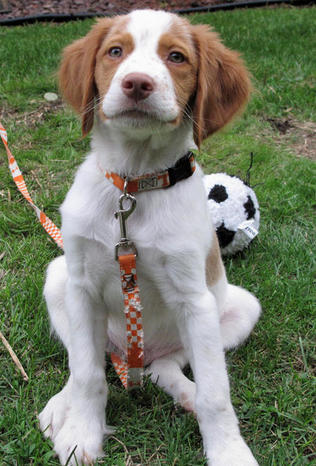
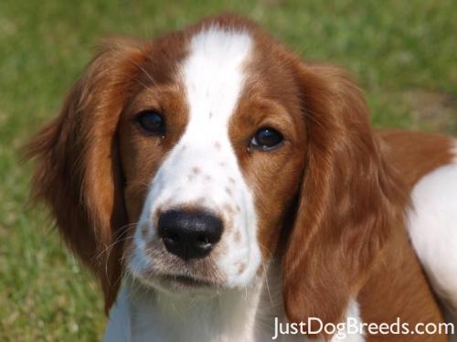
We mention that the task of assigning breed to dogs from images is considered exceptionally challenging. To see why, consider that even a human would have great difficulty in distinguishing between a Brittany and a Welsh Springer Spaniel.
| Brittany | Welsh Springer Spaniel |
|---|---|
 |
 |
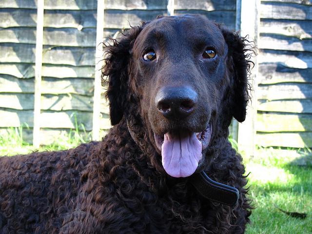
It is not difficult to find other dog breed pairs with minimal inter-class variation (for instance, Curly-Coated Retrievers and American Water Spaniels).
| Curly-Coated Retriever | American Water Spaniel |
|---|---|
 |
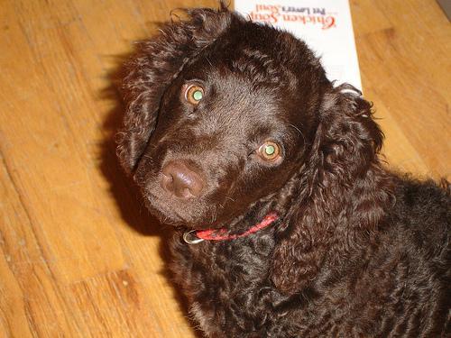 |
Likewise, recall that labradors come in yellow, chocolate, and black. Your vision-based algorithm will have to conquer this high intra-class variation to determine how to classify all of these different shades as the same breed.
| Yellow Labrador | Chocolate Labrador | Black Labrador |
|---|---|---|
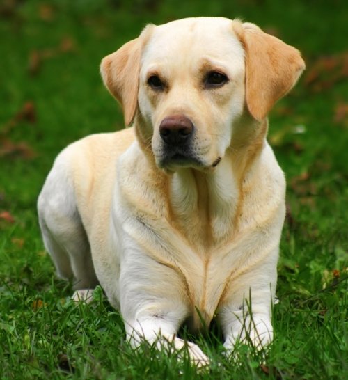 |
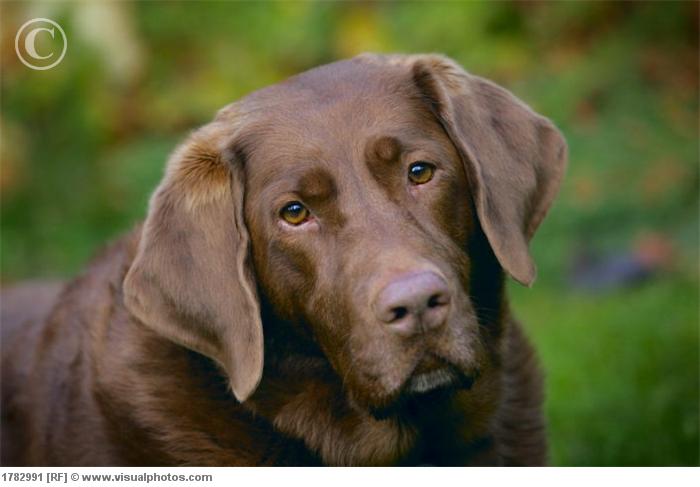 |
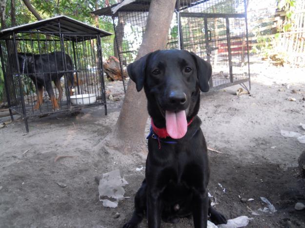 |
We also mention that random chance presents an exceptionally low bar: setting aside the fact that the classes are slightly imabalanced, a random guess will provide a correct answer roughly 1 in 133 times, which corresponds to an accuracy of less than 1%.
Remember that the practice is far ahead of the theory in deep learning. Experiment with many different architectures, and trust your intuition. And, of course, have fun!
Pre-process the Data
We rescale the images by dividing every pixel in every image by 255.
from PIL import ImageFile
ImageFile.LOAD_TRUNCATED_IMAGES = True

# pre-process the data for Keras
train_tensors = paths_to_tensor(train_files).astype('float32')/255
valid_tensors = paths_to_tensor(valid_files).astype('float32')/255
test_tensors = paths_to_tensor(test_files).astype('float32')/255
(IMPLEMENTATION) Model Architecture
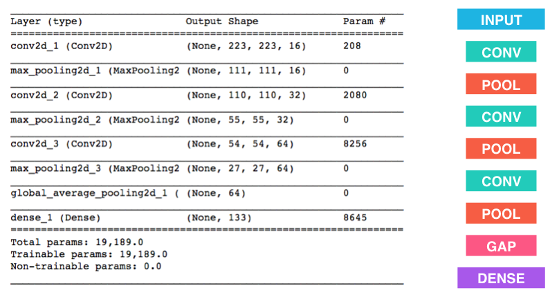
Create a CNN to classify dog breed. At the end of your code cell block, summarize the layers of your model by executing the line:
model.summary()
We have imported some Python modules to get you started, but feel free to import as many modules as you need. If you end up getting stuck, here's a hint that specifies a model that trains relatively fast on CPU and attains >1% test accuracy in 5 epochs:
Question 4: Outline the steps you took to get to your final CNN architecture and your reasoning at each step. If you chose to use the hinted architecture above, describe why you think that CNN architecture should work well for the image classification task.
Answer: When encountering an architecture problem, it's often necessary to analyze the computing resources available. The enviornment for this project is a cloud hosted p2.xlarge instance with 1 Tesla GPU which is sufficient for standard deep learning CNN architectures. The example architecture allowed for enough training and convolution to create a sufficient model. The one utilized for the initial model is similar.
The architecture begins with 3 sets of intial convolution and pooling to extract an optimal amount of paramters while maintining complexity. We use standard filter sizes of 16, kernel size of 3, and stride of 1. While the computing resources can handle a more complex architecture, there is enough resources to allow testing and experimentation of different layers. Before we output a fully connected layer, we go through 2 sets of Dropout and Dense layers because of the relatively small training size. We use the Dropout and Dense combination to adjust for possible overfitting associated with the small training size.
from keras.layers import Conv2D, MaxPooling2D, GlobalAveragePooling2D
from keras.layers import Dropout, Flatten, Dense
from keras.models import Sequential

model = Sequential()

### TODO: Define your architecture.
model.add(Conv2D(filters=16, kernel_size=3, strides=1, padding='valid', activation='relu', input_shape=(224, 224, 3)))
model.add(MaxPooling2D(pool_size=2, strides=1))
model.add(Conv2D(filters=16, kernel_size=3, strides=1, padding='valid', activation='relu', input_shape=(224, 224, 3)))
model.add(MaxPooling2D(pool_size=2, strides=1))
model.add(Conv2D(filters=16, kernel_size=3, strides=1, padding='valid', activation='relu', input_shape=(224, 224, 3)))
model.add(MaxPooling2D(pool_size=2, strides=1))
model.add(GlobalAveragePooling2D())
model.add(Dropout(0.3))
model.add(Dense(64, activation='relu'))
model.add(Dropout(0.4))
model.add(Dense(133, activation='softmax'))

model.summary()
Compile the Model
model.compile(optimizer='rmsprop', loss='categorical_crossentropy', metrics=['accuracy'])
(IMPLEMENTATION) Train the Model
Train your model in the code cell below. Use model checkpointing to save the model that attains the best validation loss.
You are welcome to augment the training data, but this is not a requirement.
from keras.callbacks import ModelCheckpoint

### TODO: specify the number of epochs that you would like to use to train the model.

epochs = 20

### Do NOT modify the code below this line.

checkpointer = ModelCheckpoint(filepath='saved_models/weights.best.from_scratch.hdf5',
                               verbose=1, save_best_only=True)

model.fit(train_tensors, train_targets,
          validation_data=(valid_tensors, valid_targets),
          epochs=epochs, batch_size=20, callbacks=[checkpointer], verbose=1)
Load the Model with the Best Validation Loss
model.load_weights('saved_models/weights.best.from_scratch.hdf5')
Test the Model
Try out your model on the test dataset of dog images. Ensure that your test accuracy is greater than 1%.
# get index of predicted dog breed for each image in test set
dog_breed_predictions = [np.argmax(model.predict(np.expand_dims(tensor, axis=0))) for tensor in test_tensors]

# report test accuracy
test_accuracy = 100*np.sum(np.array(dog_breed_predictions)==np.argmax(test_targets, axis=1))/len(dog_breed_predictions)
print('Test accuracy: %.4f%%' % test_accuracy)
bottleneck_features = np.load('bottleneck_features/DogVGG16Data.npz')
train_VGG16 = bottleneck_features['train']
valid_VGG16 = bottleneck_features['valid']
test_VGG16 = bottleneck_features['test']
Model Architecture
The model uses the the pre-trained VGG-16 model as a fixed feature extractor, where the last convolutional output of VGG-16 is fed as input to our model. We only add a global average pooling layer and a fully connected layer, where the latter contains one node for each dog category and is equipped with a softmax.
VGG16_model = Sequential()
VGG16_model.add(GlobalAveragePooling2D(input_shape=train_VGG16.shape[1:]))
VGG16_model.add(Dense(133, activation='softmax'))

VGG16_model.summary()
Compile the Model
VGG16_model.compile(loss='categorical_crossentropy', optimizer='rmsprop', metrics=['accuracy'])
Train the Model
checkpointer = ModelCheckpoint(filepath='saved_models/weights.best.VGG16.hdf5',
                               verbose=1, save_best_only=True)

VGG16_model.fit(train_VGG16, train_targets,
          validation_data=(valid_VGG16, valid_targets),
          epochs=20, batch_size=20, callbacks=[checkpointer], verbose=1)
Load the Model with the Best Validation Loss
VGG16_model.load_weights('saved_models/weights.best.VGG16.hdf5')
Test the Model
Now, we can use the CNN to test how well it identifies breed within our test dataset of dog images. We print the test accuracy below.
# get index of predicted dog breed for each image in test set
VGG16_predictions = [np.argmax(VGG16_model.predict(np.expand_dims(feature, axis=0))) for feature in test_VGG16]

# report test accuracy
test_accuracy = 100*np.sum(np.array(VGG16_predictions)==np.argmax(test_targets, axis=1))/len(VGG16_predictions)
print('Test accuracy: %.4f%%' % test_accuracy)
Predict Dog Breed with the Model
from extract_bottleneck_features import *

def VGG16_predict_breed(img_path):
    # extract bottleneck features
    bottleneck_feature = extract_VGG16(path_to_tensor(img_path))
    # obtain predicted vector
    predicted_vector = VGG16_model.predict(bottleneck_feature)
    # return dog breed that is predicted by the model
    return dog_names[np.argmax(predicted_vector)]
Step 5: Create a CNN to Classify Dog Breeds (using Transfer Learning)
You will now use transfer learning to create a CNN that can identify dog breed from images. Your CNN must attain at least 60% accuracy on the test set.
In Step 4, we used transfer learning to create a CNN using VGG-16 bottleneck features. In this section, you must use the bottleneck features from a different pre-trained model. To make things easier for you, we have pre-computed the features for all of the networks that are currently available in Keras:
- VGG-19 bottleneck features
- ResNet-50 bottleneck features
- Inception bottleneck features
- Xception bottleneck features
The files are encoded as such:
Dog{network}Data.npz
where {network}, in the above filename, can be one of VGG19, Resnet50, InceptionV3, or Xception. Pick one of the above architectures, download the corresponding bottleneck features, and store the downloaded file in the bottleneck_features/ folder in the repository.
(IMPLEMENTATION) Obtain Bottleneck Features
In the code block below, extract the bottleneck features corresponding to the train, test, and validation sets by running the following:
bottleneck_features = np.load('bottleneck_features/Dog{network}Data.npz')
train_{network} = bottleneck_features['train']
valid_{network} = bottleneck_features['valid']
test_{network} = bottleneck_features['test']# References:
# https://github.com/udacity/machine-learning/blob/master/projects/practice_projects/cnn/transfer-learning/transfer_learning.ipynb
### TODO: Obtain bottleneck features from another pre-trained CNN.
bottleneck_features = np.load('bottleneck_features/DogResnet50Data.npz')
train_Resnet50 = bottleneck_features['train']
valid_Resnet50 = bottleneck_features['valid']
test_Resnet50 = bottleneck_features['test']
(IMPLEMENTATION) Model Architecture
Create a CNN to classify dog breed. At the end of your code cell block, summarize the layers of your model by executing the line:
<your model's name>.summary()
Question 5: Outline the steps you took to get to your final CNN architecture and your reasoning at each step. Describe why you think the architecture is suitable for the current problem.
Answer: The final CCN architecture used takes advantage of the Resnet50 model available and builds upon it with additional layers. After analyzing the Resnet50 training dataset, we can conclude that the input images for dogs and humans are relatively similar. The training size for this project is relatively small. Using the matrix for transfer learning arhitecture, a small dataset with similar training data requires only a pooling layer. We apply this in our new model architecture.

### TODO: Define your architecture.
transfer_model = Sequential()
transfer_model.add(GlobalAveragePooling2D(input_shape=train_Resnet50.shape[1:]))
transfer_model.add(Dense(units= 133, activation = 'softmax'))
(IMPLEMENTATION) Compile the Model
### TODO: Compile the model.
transfer_model.compile(loss='categorical_crossentropy', optimizer='rmsprop', metrics=['accuracy'])
(IMPLEMENTATION) Train the Model
Train your model in the code cell below. Use model checkpointing to save the model that attains the best validation loss.
You are welcome to augment the training data, but this is not a requirement.
### TODO: Train the model.
checkpointer = ModelCheckpoint(filepath='saved_models/weights.best.Resnet50.hdf5', verbose=1, save_best_only=True)
transfer_model.fit(train_Resnet50, train_targets, epochs=20, validation_data=(valid_Resnet50, valid_targets),
          callbacks=[checkpointer], verbose=1, shuffle=True)
(IMPLEMENTATION) Load the Model with the Best Validation Loss
### TODO: Load the model weights with the best validation loss.
transfer_model.load_weights('saved_models/weights.best.Resnet50.hdf5')
(IMPLEMENTATION) Test the Model
Try out your model on the test dataset of dog images. Ensure that your test accuracy is greater than 60%.
### TODO: Calculate classification accuracy on the test dataset.
Resnet50_predictions = [np.argmax(transfer_model.predict(np.expand_dims(feature, axis = 0))) for feature in test_Resnet50]
test_accuracy = 100 * np.sum(np.array(Resnet50_predictions) == np.argmax(test_targets, axis = 1)) / len(Resnet50_predictions)
print('Test accuracy: %.4f%%' % test_accuracy)
(IMPLEMENTATION) Predict Dog Breed with the Model
Write a function that takes an image path as input and returns the dog breed (Affenpinscher, Afghan_hound, etc) that is predicted by your model.
Similar to the analogous function in Step 5, your function should have three steps:
- Extract the bottleneck features corresponding to the chosen CNN model.
- Supply the bottleneck features as input to the model to return the predicted vector. Note that the argmax of this prediction vector gives the index of the predicted dog breed.
- Use the
dog_namesarray defined in Step 0 of this notebook to return the corresponding breed.
The functions to extract the bottleneck features can be found in extract_bottleneck_features.py, and they have been imported in an earlier code cell. To obtain the bottleneck features corresponding to your chosen CNN architecture, you need to use the function
extract_{network}
where {network}, in the above filename, should be one of VGG19, Resnet50, InceptionV3, or Xception.
### TODO: Write a function that takes a path to an image as input
### and returns the dog breed that is predicted by the model.
def Resnet50_predict_breed(img_path):
    # extract bottleneck features
    bottleneck_feature = extract_Resnet50(path_to_tensor(img_path))
    # obtain predicted vector
    predicted_vector = transfer_model.predict(bottleneck_feature)
    # return dog breed that is predicted by the model
    return dog_names[np.argmax(predicted_vector)]
Step 6: Write your Algorithm
Write an algorithm that accepts a file path to an image and first determines whether the image contains a human, dog, or neither. Then,
- if a dog is detected in the image, return the predicted breed.
- if a human is detected in the image, return the resembling dog breed.
- if neither is detected in the image, provide output that indicates an error.
You are welcome to write your own functions for detecting humans and dogs in images, but feel free to use the face_detector and dog_detector functions developed above. You are required to use your CNN from Step 5 to predict dog breed.
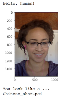
Some sample output for our algorithm is provided below, but feel free to design your own user experience!
(IMPLEMENTATION) Write your Algorithm
### TODO: Write your algorithm.
### Feel free to use as many code cells as needed.
def classify(img_path) :
    # If dog is detected, return the dog breed
    if (dog_detector(img_path)) :
        print "Dog Detected.\nResembling Breed: {}\n".format(Resnet50_predict_breed(img_path))
    elif (face_detector(img_path)) :
        print "Human Detected.\nResembling Dog Breed: {}\n".format(Resnet50_predict_breed(img_path))
    else :
        print "Neither human nor dog detected.\n"
Step 7: Test Your Algorithm
In this section, you will take your new algorithm for a spin! What kind of dog does the algorithm think that you look like? If you have a dog, does it predict your dog's breed accurately? If you have a cat, does it mistakenly think that your cat is a dog?
(IMPLEMENTATION) Test Your Algorithm on Sample Images!
Test your algorithm at least six images on your computer. Feel free to use any images you like. Use at least two human and two dog images.
Question 6: Is the output better than you expected :) ? Or worse :( ? Provide at least three possible points of improvement for your algorithm.
Answer: The output is relatively accurate and the following analysis describes each image,
ariana.jpg- Subject: Celebrity pop star Ariana Grande
- Model Classification: Neither
- Comments: The image was chosen to test the classification based on the cat ears worn by the subject. There could be multiple reasons for the classification including an unclear view of the face or because the subject depicts a human with cat ears which can be vague. The model is reasonable with the output.
beagle.jpg- Subject: Beagle
- Model Classification: Dog, Beagle
- Comments: This image was a clear depiction of a beagle where most dog owners are familiar with this breed. The inital detector was able to accurately identify the general subject and then the model was able to pinpoint the subclassification or breed. The model is accurate with the expected output.
cup.jpg- Subject: Empty cup and plate
- Model Classification: Neither
- Comments: The image was chosen to test the classification based on arbritary subjects not humans or dogs. The detectors did not recognize it as a positive result. This is the expected output.
golden_retriever.jpg- Subject: Golden Retriever
- Model Classification: Dog, Golden Retriever
- Comments: This image was a clear depiction of a golden retriever also one of the most recognizable dog breeds. he inital detector was able to accurately identify the general subject and then the model was able to pinpoint the subclassification or breed. The output for this test is accurate.
hammad.jpg- Subject: Me
- Model Classification: Human
- Comments: The image was chosen to test the classification of my own portrait. The detector was able to confirm that I'm a human instead of a dog or neither, in the case of Ariana Grande with cat ears. The face detector is accurate 98% of the time for true positives based on the accuracy measurements calculated earlier. Out of curiosity, the model classified me resembling most with a Silky Terrier dog.
toulouse.jpg- Subject: Ariana Grande's Chihuahua mix
- Model Classification: Dog, Afghan Hound
- Comments: The subject is a mix between a Chihuanhua and a Beagle and was chosen to see the model's classification of mixed breed animals. The detector correctly identified it as a dog but the model for classification wasn't able to accurately describe the dog breed. An Afghan hound is a much larger dog compared to the subject in the picture but could be due to the smaller training size.
Possible Improvements:
References:
- https://machinelearningmastery.com/improve-deep-learning-performance/
- https://blog.keras.io/building-powerful-image-classification-models-using-very-little-data.html
Larger Data Set: The provided training data set is relatively small compared to other data sets that can provide additional training and testing. With a larger data set we have more data points to learn from. If we can double the number of images to a range of 15,000 to 16,000 than this can increase our model's performance.Augment Training Data: Augmenting the data set was suggested as optional but it can help us create a better training data set. This includes transforming the images so they are normalized and applying random transformations to create additional data. By augmenting the images, we are able to train image optimally rather than training on the raw images.Algorithm Tuning: We're able to utilize the full breadth of parameters in a convolutional nerual network which includes batch size, kernel size, number of epochs, etc. to output a model with the best performance. Within the context of our problem, the parameters that can provide optimized performance are learning rate, number of epochs, and number of filters. The learning rate and number of epochs are closely related to how the model learns from the training data set where the lower and the learning rate and larger the number of epochs, the greater potential performance we can achieve. A greater number of filters affects the architecture of our nerual network and can also allow the model to output with greater performance.
## TODO: Execute your algorithm from Step 6 on
## at least 6 images on your computer.
## Feel free to use as many code cells as needed.
from IPython.display import Image, display
dataset = ['ariana.jpg', 'beagle.jpg', 'cup.jpg', 'golden_retriever.jpg', 'hammad.jpg', 'toulouse.jpg']
for img in dataset :
    print(img)
    img_path = 'test/{}'.format(img)
    display(Image(filename = img_path, width = 100))
    classify(img_path)


